5. Dynamics#
5.1. Introduction#
In statics we study forces on a rigid body, the forces being balanced so that the body is at rest or moving at a constant speed. In dynamics we study the movement of a rigid body, on which forces act that are not balanced. There is a resulting force that causes acceleration and therefore a change in velocity and position.
The difficulty here is that the forces themselves can depend on the velocity or position of the body. Consider, for example, a car where the air resistance depends on the velocity of the car or where a bump in the road influences movement.

Fig. 5.1 (a) Racing car, (b) dynamic model of a (racing) car.#
With a so-called dynamic model, see Fig. 5.1 (b), we try to describe the relationship between forces, accelerations, velocities and displacements, which form the information to investigate the ultimate movement of the object, for example the car. This movement analysis can be the basis for the design of a suitable wheel suspension, but also, for example, to be able to compensate for unwanted vibrations in a machine (part). They also form the starting point for designing a control scheme (see Section 6).
A very different example of applying dynamics is the motion analysis of a drill rod and drill bit, see Fig. 5.2. A dynamic model was used to gain insight into the way in which frictional forces on a drill bit at the bottom of a kilometer-long drill rod influence the rotation of this drill rod.

Fig. 5.2 Drilling rig.#
In this chapter you will become acquainted with the principles of dynamics. A typical example from the dynamics is the mass-spring-damper system. In this chapter we investigate the movement of a simple mass-spring-damper system.
5.2. Mass, force and acceleration#
5.2.1. Newton’s second law#
The basic principle of dynamics is Newton’s second law. Newton’s second law describes the relationship between force and acceleration, which in turn is related to the change of velocity and position of the rigid body. Consider a mass \(m\) moving under the influence of a resulting force \(F\), so these are all forces acting on the mass \(m\). Note that the force \(F\) is generally a vector, a quantity with a certain length and direction.

Fig. 5.3 Mass \(m\) moves under the influence of force \(F\).#
The acceleration \(a\) that the mass gets is described by Newton’s second law:
in which \(\sum F\) is the resulting force in [N], \(m\) the mass in [kg] and \(a\) the acceleration in [\(\textrm{m}/\textrm{s}^2\)]. The acceleration is equal to the velocity change per unit time, or \(\displaystyle a=\frac{dv}{dt}=\dot{v}\). In which \(\dot{v}\) (pronounced: v-dot) is the first derivative of the velocity. In turn, the velocity is the position change per unit time, or \(\displaystyle v=\frac{dx}{dt}=\dot{x}\).
Finally, we can write for acceleration \(a\):
In which \(\ddot{x}\) (pronounced: x-double-dot) is the second derivative of \(x\). Newton’s second law can then be written as:
Because the twice differentiated position \(\ddot{x}\) occurs in (5.3), we call (5.3) a second-order differential equation.
5.2.2. Acceleration, velocity and position#
If the velocity in the time interval [0, \(t\)] is known, then the change in position (displacement \(x\)) during that time interval can be calculated by integration. If the starting position at \(t=0\) is also known, the position can be determined. This can sometimes be done graphically, as in Fig. 5.4, where the area under the \(v(t)\)-graph is equal to the displacement \(\Delta x(t)\).

Fig. 5.4 The area under the v(t)-graph is the displacement \(\Delta x(t)\).#
This can sometimes also be done analytically, provided that the velocity is known as a mathematically described function of time. For a single movement (constant velocity) this can be described as follows:
If the velocity over time is unknown, but the acceleration is known, then the velocity change can be determined by integrating the acceleration over time. With the initial velocity \(v(0)\), the velocity \(v(t)\) over time can be determined. If the starting position \(x(0)\) is known, the position \(x(t)\) can be determined by integration of the velocity. It is possible to do this graphically. It can also be done analytically, provided that the acceleration, as a function of time, is given. Fig. 5.5 shows the relationship between acceleration, speed and position schematically.

Fig. 5.5 The relationship between acceleration, velocity and position.#
For a uniformly accelerated movement (constant acceleration) the following can be stated:
Analytical determination of acceleration and speed
The position of a car is described by a mathematical function. This function was determined by performing many position measurements during the movement and fitting a function through it. The final function is equal to:
Find an expression for the velocity and acceleration of the car over time.
Solution
The velocity and acceleration can be determined by differentiating the position-time function to time:
Analytical determination of position and velocity
In a second experiment, it is not the position but the acceleration of a car that is measured. Again, a mathematical connection has been fitted through the experimental data. The relationship found is equal to:
Find an expression for the velocity and position of the car over time. It is stated that the initial velocity \(v(0) = 15\, \textrm{m/s}\) and that the initial position \(x(0) = 150\, \textrm{m}\).
Solution
The velocity and position can be determined by integrating the acceleration-time function:
With the initial condition: \(v(0) = 15\, \textrm{m/s} \to C = 15\).
Tachograph
Touring buses and trucks nowadays contain tachographs. These register the velocity over time at which the coaches and trucks drive. The \(v-t\) graph below has been derived from such a tachograph over a time interval of 12 seconds.

Fig. 5.6 \(v-t\) graph.#
Determine graphically the displacement and the acceleration as a function of time.
Solution
The displacement as a function of time can be deduced by determining the area under the \(v-t\) graph. The total displacement is equal to the area under the graph, thus
The velocity change can be seen in the \(x-t\) graph, the steepness of the \(x-t\) graph goes from \(30 \textrm{m}/\textrm{s}\) to \(0 \textrm{m}/\textrm{s}\) and back again to \(30 \textrm{m}/\textrm{s}\).

Fig. 5.7 Proceedings of displacement and acceleration.#
The acceleration as a function of time can be deduced from the velocity-time graph by determining the steepness of the graph. \(t \in [0,2]\) and \(t \in [10,12]\) the derivative is zero.
For \(t \in [2,6]\) the acceleration is negative, namely \(\textrm{a} = -7.5 \, \textrm{m/s}^2\). For \(t \in [6,10]\) the acceleration is positive, \(7.5\, \textrm{m/s}^2\). At \(t=6\) the acceleration suddenly changes sign.
5.3. Mass-spring system#
In many cases, the force that acts on a mass is not constant. A common example of a non-constant force is the spring force. The force required to stretch a spring depends on its extension. We consider a linear spring here. In addition, the required force is proportional to the elongation: \(F_k = k \cdot (l-l_0)\), where \(l_0\) is the length of the relaxed spring. The relaxed length \(l_0\) is the length of the spring when no force is applied to the spring.

Fig. 5.8 Force required to stretch a linear spring.#
We consider a mass m which is attached to the fixed world via a spring with stiffness \(k\) and relaxed length \(l_0\). The position \(x\) of the mass is measured. If the spring is in the relaxed state, \(x\) equals 0, or: \(x = l - l_0\).

Fig. 5.9 Mass-spring system.#
We are interested in the position of the mass over time if we give the spring at \(t=0\) an extension \(x_0\) of: \(x(t=0) = x_0\). Fig. 5.9(b) shows the forces that act on the mass \(m\).
We write down Newton’s second law:
The spring force \(F_k\) is directly proportional to the elongation of the spring, or to the displacement \(x\), \(F_k = k \cdot x\), where \(k\) represents the stiffness with dimension [N/m]. Using these relations and combining with (5.2) and (5.6) this becomes:
In which \(\ddot{x}\) is an abbreviated notation for the second time derivative of \(x\), see ((5.3)). We call the resulting equation a differential equation. Using Calculus it can be explained how you can solve such an equation. For now, we will suffice with giving the solution. A possible solution of ((5.7)) is:
In this equation we call \(\omega\) the eigen frequency of the mass-spring system. With \(x(0) = x_0\) and v(0) = 0, \(A = x_0\) and \(B = 0\).
Now equation (5.8) is changed to:
Note
Check that this solution complies with equation (5.7), by entering the solution ((5.8)) and its second-order derivative in ((5.7)) and checking the initial condition.
If we plot position \(x\) and the velocity \(v=\frac{dx}{dt}=\dot{x}\) against time, we get the following graphs. These graphs describe the response of the mass-spring system to an initial stretch of \(x_0\) and an initial velocity of \(\dot{x}_0=0\). The response is periodic: after every vibration time \(T (= 2\pi/\omega)\) the response is repeated.

Fig. 5.10 Response of a mass-spring system.#
A special way to display the response of a dynamic system is the so-called phase plane. In the phase plane we plot the displacement \(x\) and the velocity against each other. The response in the phase plane shows, in a well-arranged manner, which positions and speeds can occur for a certain initial condition.
The position \(x\) can therefore be a sum of two vibrations with different amplitudes \(A\) and \(B\). Here, these vibrations do have the same frequency, but a different starting point. The one is then sine-shaped, the other cosine-shaped.
Fig. 5.11 shows the mass-spring system response in the phase plane for different starting positions \(x_0\) and \(v_0 = \dot{x}_0 = 0\).

Fig. 5.11 Response of the mass-spring system in the phase plane for \(x(t) = x_0 \cdot \cos(\omega \cdot t)\).#
At \(t = 0\) the position is \(x = x_0\) and the velocity is \(\dot{x} = 0\). After \(0.25 \textrm{ T}\), the displacement \(x = 0\) and the velocity is maximum (negative): \(\dot{x} = -\omega\, x_0\). This can be seen from Fig. 5.10. At \(t = 0.5 \textrm{ T}\) the elongation is maximum (negative): \(x = -x_0\) and the velocity \(\dot{x}= 0\). After \(T\), the system is back in the initial state.
Car suspension
We consider the theoretical case of a car including passengers (\(m = 1000\, \textrm{kg}\)) without damping in the suspension. We consider the suspension as linear. The four springs together have a stiffness \(k\) of \(10^6\, \textrm{N}/\textrm{m}\). For \(t< 0 \), the car is at rest, the bottom of the car is \(0.10\) meters from the ground (\(x = 0.10\, \textrm{m}\)).

Fig. 5.12 Car with suspension.#
Then 4 passers-by push the car down with their own weight (250 kg). They release the car at \(t = 0\, \textrm{s}\). The car starts to vibrate.
Calculate the extra sagging of the car when it is pushed down. At what height from the floor is the bottom of the car, just before the passers-by let it go?
Solution
At \(t = 0\) the four passers-by press on the car with 250 kg, this causes the suspension to sag further. The extra sagging is equal to:
The bottom of the car is now at \(x = 100\, \textrm{mm} - 2.45\, \textrm{mm} = 97.55\, \textrm{m}\) from the ground.
After releasing the car will vibrate. The height of the car bottom as a function of time can be written as follows:
Where \(x(t)\) is the height of the car bottom in [mm], \(x_s\) the stationary sagging (equilibrium position) in [mm], \(m\) the mass of the car + passengers in [kg] and \(k\) the combined stiffness of the suspension in [N/m]. Determine the constants \(x_s\), \(A\) and \(\omega\).
Solution
After the car is released, it starts vibrating.
Given is the response of the bottom of the car (with \(x_s\) as stationary final position):
For the equilibrium position, the following applies: \(x_s = 100\, \textrm{mm}\).
At \(t = 0\, \textrm{s}, x = 97.55\, \textrm{mm}\). Substituting \(t = 0\) gives:
With \(m = 1000\, \textrm{kg}\) and \(k = 10^6\, \textrm{N/m}\), the angular frequency \(\omega\) of the vibration becomes:
The response is therefore:. With \(x(t)=100-2.45 \cdot (31.6 t)\). With \(x(t)\) the height of the car bottom in \(\textrm{mm}\).
Draw the response of the car in the phase plane.
Solution
From the car bottom height as a function of time we can determine the velocity of the car bottom as a function of time:
We calculate the height and velocity of the car floor at a different instances in time. Based on this, we draw the response in the phase plane.
\(t\ [\textrm{s}]\) |
\(x\ [\textrm{mm}]\) |
\(t\dot{x}\ [\textrm{mm/s}]\) |
|---|---|---|
\(0\) |
\(100 - 2.45 = 97.55\) |
\(0\) |
\(0.25 T = 0.05\) |
\(100\) |
\(77.5\) |
\(0.5 T = 0.10\) |
\(100 + 2.45 = 102.45\) |
\(0\) |
\(0.75 T = 0.15\) |
\(100\) |
\(-77.5\) |
\(T = 0.20\) |
\(100 - 2.45 = 97.55\) |
\(0\) |

Fig. 5.13 Response of the car and suspension in the phase plane.#
5.4. Mass-spring-damper system#
In reality, every spring is damped. By that we mean that the vibration of the mass and the spring eventually diminishes. The response, as drawn in Fig. 5.10, then looks, for example, as in Fig. 5.14.

Fig. 5.14 Damped vibration.#
The video below shows an experiment of a 1 Degree of Freedom Spring-Mass-Damper system. Real springs exhibit dissipative effects, modelled as a damper. In the experiment, the oscillation’s amplitude decays exponentially, while the frequency remains constant.[1]
We can model this damping by adding a linear damper in addition to the linear spring. With a linear spring, the force required to stretch the spring is directly proportional to the spring extension. With a linear damper, the force required to “stretch” the damper is directly proportional to the velocity difference of the two ends of the damper. Fig. 5.15 shows a damper that is attached to the fixed world on one side. The force required to move the damper is directly proportional to the velocity of the damper end.

Fig. 5.15 Damping force.#
If you want to move the damper in Fig. 5.15 quickly, you need a large force. If you do it slowly you need a small force. Some trunks of cars are equipped with gas dampers. If you open the trunk quickly it costs more force than if you do it slowly.
Fig. 5.16(a) shows a mass that is attached to the fixed world with a spring and a damper. The position \(x\) and the velocity of the mass are measured. When the spring is in the relaxed state, \(x = 0\).

Fig. 5.16 Mass-spring-damper system.#
Again, we are interested in the position of the masses over time if we give the whole system an initial stretch of \(x_0\) and then let go. The forces on the mass are shown in Fig. 5.16(b). Writing down Newton’s second law for this mass gives
The spring force is directly proportional to the displacement \(x\) of the mass: \(F_k = k \cdot x\). The damper force is directly proportional to the velocity of the mass: \(F_d = d \cdot \dot{x}\).
The acceleration a of the mass is equal to the second-order derivative of the displacement: \(a=\ddot{x}\).
With that information (5.10) changes to:
The solution of this differential equation is somewhat more complicated than that of (5.7). In fact, depending on the (mutual ratio) of the value of the parameters \(m\), \(d\) and \(k\), there are even two different types of solutions. We call these different solutions under or over critically damped.
To make this easier to see, differential (5.11) is often rewritten in a different form. In this equation, the parameters \(m\), \(d\) and \(k\) are replaced by the two important key parameters \(\omega_n\) and \(\zeta\).
With \(\omega_n\) the undamped eigenfrequency and \(\zeta\) the damping ratio.
We can recognize the undamped eigenfrequency \(\omega_n\) from the mass-spring system of (5.7). The damping ratio is a parameter that says something about the influence of the damping.
Use (5.12) to derive the expressions for n and from (5.13).
Tip
\(m\ddot{x} + d \dot{x} + kx = 0 \to \ddot{x} + \frac{d}{m}\dot{x}+ \frac{k}{m}x = 0 \to 2 \zeta \omega_n \quad \text{and} \quad \frac{k}{m}=\omega_n^2\)
There are two different solutions depending on the value of \(\zeta\). Compare the following two examples.
5.4.1. Underdamped systems#
If we add a relative “weak” damper to the mass-spring system of (5.7), you can imagine that the system will vibrate periodically, but that the amplitude of that vibration will slowly be damped.
For \(\zeta < 1 \), the solution of differential (5.11) can be written in the following form (with initial condition for the position \(x(t=0) = x_0\) and for the velocity \(\dot{x}(t=0)=\dot{x}_0=0\)):
This clearly shows that the amplitude of the vibration as a function of time decreases according to a e to the power. It is also striking that the angular frequency of the vibration is no longer the same as the undamped eigenfrequency. That is why \(\omega_d\) is called the damped eigenfrequency.
The response of the displacement and velocity against time will then look like this:

Fig. 5.17 Response of a under critically damped mass-spring-damper system.#
In the interactive figure below you can move the slider to adjust the value of \(\zeta\) between 0 and 1 to see the displacement \(x\) of the mass as a function of time \(t\).
5.4.2. Overdamped systems#
In a system with a relatively strong damper, you can imagine that there is no periodic vibration, but that the system just moves slowly to its equilibrium point (such as the trunk of the car with the gas damper). Such a system is often overdamped. In dynamics we are talking about an overdamped system when \(\zeta > 1\). The response, and therefore the solution of differential (5.11), can then be written as:
In this equation \(\lambda_1\) and \(\lambda_2\) are only depending on m, d en k, while A and B are defined by the initial conditions \(x(t=0) = x_0\) and \(\dot{x}(t=0)=\dot{x}_0\).
The response of the displacement and the velocity against time then looks like this:

Fig. 5.18 Response of an overdamped mass-spring-damper system.#
Because there are no longer sine or cosine terms in the response, the mass in an overdamped system does not perform periodic vibration. If we plot the response for both systems in the phase plane, we get:

Fig. 5.19 Response in the phase plane of a (a) overdamped and (b) underdamped system.#
The video below shows the phase plane for an underdamped system. Displacement, \(x\), of the spring mass damper system is on the \(x\)-axis and the velocity, \(v\), is on the \(y\)-axis. The vector field is generated from the equation of motion: \(\displaystyle \frac{dx}{dt} = v \) and \(\displaystyle \frac{dv}{dt} = -(k/m)x - (d/m)v\), where \(k\) is the spring stiffness, \(d\) is the damping coefficient, \(m\) is the mass, \(t\) is time.[1]
Note
Verify that the response in the phase plane of Fig. 5.19(a) and (b) corresponds to the responses against time in respectively Fig. 5.18 and Fig. 5.17.
Under or overdamped?
We consider a mass-spring-damper system that is described by differential (5.12). It is given that \(\dfrac{d}{m} = 3\) and \(\dfrac{k}{m} = 2\).
Is the system over or underdamped?
Solution
In order to check whether the system is over or underdamped, we must determine the damping factor \(\zeta\). We derive the following from (5.13):
The damping ratio is higher than 1, therefore the system is overdamped.
The response is given as follows: \(x(t) = Ae^{-t} + Be^{-2t}\), with \(x(t)\) in [m].Determine the constants \(A\) and \(B\), if the starting position is \(x(t=0)=5\) [m] and the starting velocity \(\dot{x}(t=0)=0\, \textrm{m/s}\).
Solution
The proposed response corresponds to the response of an overdamped system. We get the response of the velocity by differentiating:
To comply with the initial conditions, the following must be true (\(t=0)=5\, \textrm{m}\) and \(\dot{x}(t=0)=0\, \textrm{m/s}\).
Solving this system gives: \(A=10\, \textrm{m and } B=-5\, \textrm{m}\).
5.5. Non-linear dynamic systems#
In the previous sections we have assumed linear springs and dampers. Here, the spring force was proportional to the elongation and the damper force proportional to the difference in velocity of the damper ends. In practice, springs and dampers only have a small part in which they are linear. For example, most springs will become weaker if they stretch more.
Fig. 5.20 shows how the spring force against the elongation could look like. It is clear that the spring is not linear.

Fig. 5.20 Spring force against elongation with a non-linear spring.#
The response of a non-linear system can take all kinds of typical forms. Fig. 5.21 shows an example of a response from a non-linear system.

Fig. 5.21 Example of non-linear response (a) against time, (b) in the phase plane.#
Characteristic of the response of non-linear systems is that, among other things, multiple equilibrium points or periodic solutions can be found. In many cases, the solutions of a non-linear system even behave chaotically; over time, the solution can become completely unpredictable.
In the context of this course you do not have to be able to work with non-linear dynamic systems.
5.6. What lies ahead#
In this chapter a few simple examples from dynamics are discussed. It is essential that, using physical laws, the movement of a mass (e.g. a car) is described by a differential equation. A relationship is given between position, velocity and acceleration of the mass.
With a more complicated mechanical system, the description is more difficult and may consist of a coupled system of differential equations. Just think of several masses that are connected via with springs and dampers. In such a case, setting up the system of differential equations is not easy, while analyzing or determining the solutions is a challenge in itself. Nevertheless, with the help of numerical methods and quantitative analysis, much insight can be gained about the system. In this way you can, among other things, try to understand how the drill bit (Fig. 5.2) moves at the end of a kilometer-long drill rod. Or how much the Erasmus bridge (Fig. 5.22) vibrates under the influence of the wind.

Fig. 5.22 Erasmus bridge.#
In this chapter you only became acquainted with the response of linear springs and dampers. The research field of non-linear dynamics is particularly concerned with the non-linear behavior of dynamic systems. Almost all mechanical systems are non-linear, but in many cases it is sufficient to assume that the description is approximately linear. Certainly in the case where we want a very accurate description of a mechanical system, we can no longer make such an approach. Just think for instance about the ever-occurring friction in a mechanical system or about a mobile robot.
In this chapter you have only considered a dynamic system that consists of one mass, one spring and one damper. In practice, there are numerous systems (such as robots) that in modeling consist of many masses, springs and dampers. Computer support plays a major role in analyzing such systems. Analyzing systems that contain multiple moving masses (or bodies) is called the research area of multi-body dynamics. A model of a dynamic system is not only of great importance for the dynamic analysis of the system, but also for the design of controllers.
5.7. Problems#
For the following exercises use symbols as long as possible and only in the end fill in the values given.
Exercise 5.1 (CD-player in car)
We consider a cd-player installed in a car. The driver notices that the cd jumps when driving on a rough road, i.e. the player does not deliver the correct signal. He decides to investigate this. He dismounts the cd-player from the car, and inserts a cd. By means of a laser-measuring technique he determines the distance between the read surface of the cd and the reading head of the laser. This distance is \(9.0\, \textrm{mm}\) for the system in equilibrium. Next, the researcher hits the cd-player. Below you find the evolution of the distance \(h\) between the read surface of the cd and the reading head of the laser as a function of time.

Fig. 5.23 Evolution of the distance between the read surface of the cd and the reading head of the laser.#
Is this an under- or overdamped system? Motivate your answer.
Sketch qualitatively the response in the phase plane (so a \(\displaystyle \frac{dx}{dt}\)-\(x\)-diagram). Representing velocities qualitatively suffices (there is no need to calculate velocities).
The weight of the oscillating mass \(m = 16.0\, \textrm{gram}\). From the response in Fig. 5.23 the damping factor \(\zeta = 0.128\) has been determined.
Determine from the diagram in Fig. 5.23 the angular frequency with which the cd oscillates in [rad/s].
Determine the damping constant \(d\) in [\(\textrm{Ns}/\textrm{m}\)] and the spring constant \(k\) in [\(\textrm{N}/\textrm{m}\)] of the mounting.
What is the minimal damping constant \(d\) (for unaltered \(k\) and \(m\)) to make the cd come to a standstill monotonously, i.e., without oscillation?
Context
The subject of both next exercises is a printer. Positioning the printer head is crucial for a good functioning of the printer. This positioning determines where the ink is deposited on the paper. Besides the position accuracy requirements that follow from this, also the speed at which accurate positioning takes place is important.

Fig. 5.24 Views of a printer head.#
Research and design questions
Consider the following design questions:
How fast can we position the printer head?
Which system properties play an important role in this?
Exercise 5.2 (Positioning of a printer head)
The printer head should be positioned in the middle. To that end, the toothed belt (and therefore the printer head mounted on it) is set in motion by means of a motor. By means of a model of the dynamics we investigate how the position \(x\) of the printer head evolves over time \(t\). The parts of the tooted belt, left and right of the printer head, are modelled as a spring \(k\) and damper \(d\), see Fig. 5.25.

Fig. 5.25 Model of a printer head. Top: actual representation. Bottom: represented as a mass-spring-damper-system.#
Four forces act on the printer head: two spring forces and two damping forces, see Fig. 5.26. If the printer head is exactly in the middle, we have \(x = 0\). In that case both springs are in their relaxed position with length \(l_0\). If the printer head is entirely on the left, we have \(x = -l_0\). If the printer head is entirely on the right, we have \(x = l_0\).
Below you see how the printer head is isolated (free body diagram) and how the spring and damper forces have been defined.

Fig. 5.26 Model of the printer head; printer head isolated.#
Parameters |
|
|---|---|
\(m\) |
The mass of the printer head in [kg]. |
\(k_1\) |
The stiffness of the left part in [\(\textrm{N}/\textrm{m}\)]. |
\(k_2\) |
The stiffness of the right part in [\(\textrm{N}/\textrm{m}\)]. |
\(d_1\) |
The damping of the left part in [\(\textrm{N}\textrm{s}/\textrm{m}\)]. |
\(d_2\) |
The damping of the right part in [\(\textrm{N}\textrm{s}/\textrm{m}\)]. |
\(x\) |
The position of the printer head with respect to the middle in [m]. |
\(\frac{dx}{dt}\) |
The velocity of the printer head in [\(\textrm{m}/\textrm{s}\)]. |
Show that for the spring lengths: \(l_1 = l_0 + x\) and \(l_2 = l_0 - x\).
Derive from this that the spring forces are given by: \(F_{k,1} = k_1\, x\) and \(F_{k,2} = -k_2\, x\). Both with respect to the positive directions as depicted in Fig. 5.26.
Show by means of Newton’s 2nd law that the resulting differential equation is given by
From measurements it is known that \(k_1 = k_2 = 3.5\cdot 10^4 \textrm{ N}/\textrm{m}\), \(d_1 = d_2 = 6.75 (\textrm{ N}\, \textrm{s})/\textrm{m}\) and \(m = 0.250\) kg.
Determine the undamped eigenfrequency \(\omega_n\), the dimensionless damping ratio \(\zeta\) and the damped eigenfrequency \(\omega_d\). Is the system under- or overdamped? Does the printer head come to a standstill with oscillation?
The printer head should be positioned in the middle at \(x_{\textrm{final}} = 0\). At \(t = 0\) the printer head reaches \(x_{\textrm{final}}\) and the motor is stopped immediately. The printer head still has a velocity of \(\frac{dx}{dt} = \dot{x} = 1 \textrm{ m}/\textrm{s}\).
The motion of the printer head as a function of time is given by
Check that this solution meets the initial conditions at \(t = 0\) s. Draw the solution \(x\) as a function of time \(t\).
Suppose that the printer head can only eject ink to the paper when the amplitude of the movement of the printer head (with respect to the paper) is less than \(\Delta x\). First determine the amplitude as a function of time.
At what time instance can the printer head eject ink to the paper, when \(\Delta x = 1.0\cdot 10^{-4}\) m (\(=0.10\) mm) is required?
extra
Exercise 5.3 (Optimisation of the printer head)
Investigate the effect of modifying the system parameters to the above defined time instance in equation (5.17), and therefore to the “speed” with which the printer can operate.
What is the effect of a twice as heavy printer head?
What is the effect of a twice as stiff toothed belt (\(k_1\) and \(k_2\) are doubled)?
What is the effect of a toothed belt which has twice as much damping (\(d_1\) and \(d_2\) are doubled)?
The printer head in this exercise needs \(0.11\) seconds per movement to stop oscillating. If the printer head can print \(1\) character per movement, printing one line takes \(10\) seconds, which is way too long. To increase the printing speed, one could reduce the mass of the printer head, stiffen the toothed belt, or increase the damping (by selecting a different material).
In practice, a large improvement can be achieved by means of a controller. The controller makes sure that when approaching its final destination the printer head gradually decelerates, instead of suddenly turning of the motor. In this way the final oscillation is reduced considerably.
Exercise 5.4 (Balance masses)
Without a vibration isolation system, vibrations generated in one part of a system can directly travel towards the ground and/or other parts of the system. The dynamics of this are visualised in Fig. 5.27 and Fig. 5.28. This can subsequently affect the proper functioning of those nearby systems and/or other parts in the system.
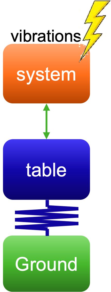
Fig. 5.27 Shows vibration transfer from the system through the table into the ground without isolation, allowing vibrations to move freely between components.#
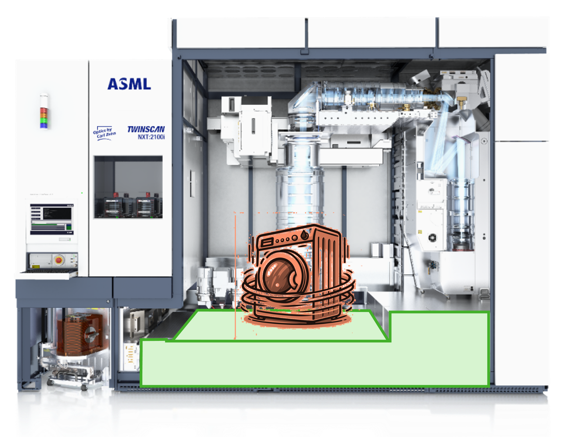
Fig. 5.28 Depicts a precision ASML machine where internal vibrations can travel through the structure to the ground and surrounding systems if not isolated. The system in orange is concidered as the position module where in green the base frame is shown.#
With a vibration isolation system, e.g., a balance mass, vibrations generated in one part of a system are “absorbed” by the balance mass. Consequently, the surroundings (inside and outside the system) hardly feel anything of the original vibrations. The dymanics of this can be seen in Fig. 5.29 and Fig. 5.30.
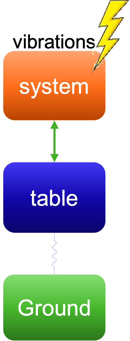
Fig. 5.29 Shows vibration isolation using a balance mass that absorbs motion forces, preventing vibrations from reaching the ground.#
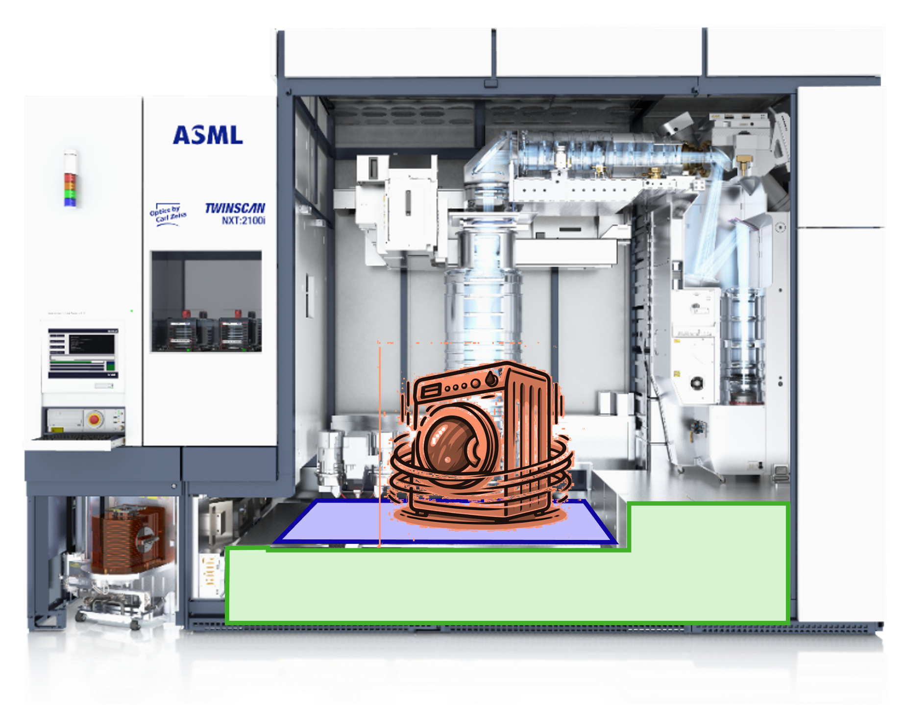
Fig. 5.30 Depicts the ASML machine with an integrated balance mass structure (in blue) that confines vibrations within the system, minimizing transmission to the surroundings. The system in orange is concidered as the position module where in green the base frame is shown.#
Let us consider the wafer stage module in ASML lithography systems shown in Fig. 5.32 as an exercise of how a balance mass works. The position module pushes against the balance mass when it moves, i.e., when it generates disturbance vibrations. In this exercise, we analyze how an ideal balance mass works, and how the balance mass behavior is affected by design constraints. A schematic representation of the high-lighted parts is given below in Fig. 5.31.

Fig. 5.31 Illustrates the interaction between the position module (in orange) and balance mass (in blue), where motion forces from the moving module are counteracted by the balance mass to minimize vibration transfer to the base frame (in green).#
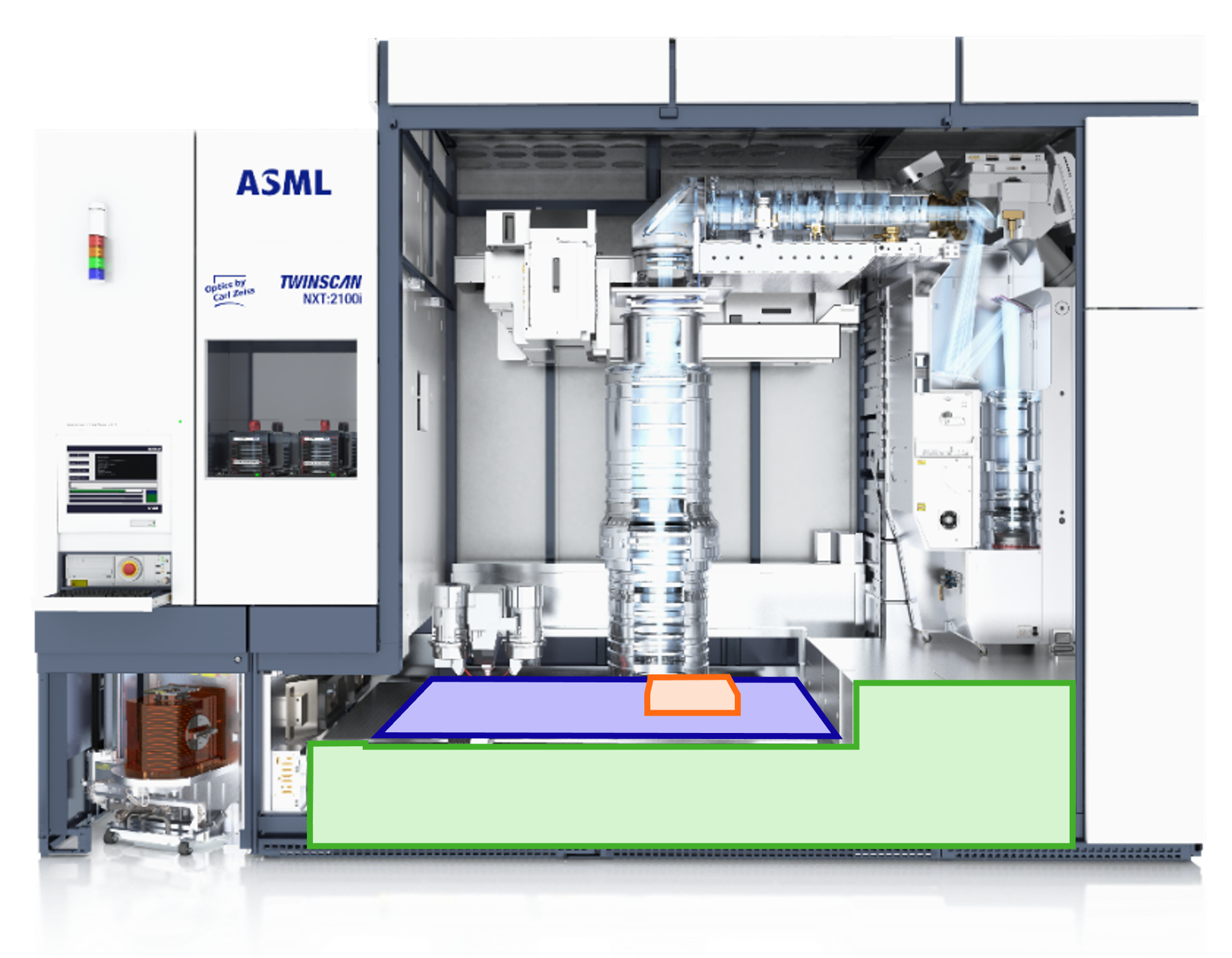
Fig. 5.32 Shows the ASML lithography system highlighting the wafer stage composed of the position module (in orange) and balance mass (in blue) mounted on the base frame (in green), which acts as the fixed reference.#
Assume motors on the position module generate a force \(F_{\rm mov}\) in positive \(x\) direction, what is then amplitude and sign of the force \(F_{BM}\) felt by the balance mass?
Based on Newton’s second law, we know that \(F = m \ddot{x}\). Assume that initially the position module and balance mass both are at rest at position \(0\, \rm m\) (see Fig. 5.33). Then given a constant force \(F_{\rm mov}\), derive the displacements of the two bodies as function of time.
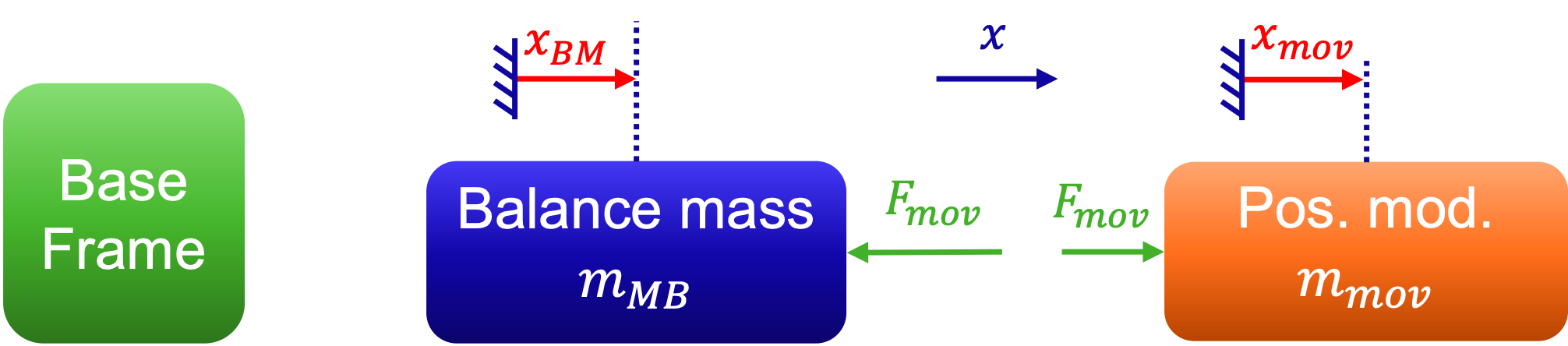
Fig. 5.33 The simplified dynamic model of where the motion of the position module and balance mass are related through Newton’s second law, illustrating force interaction and displacement ratio analysis.#
Give an expression for the ratio \(x_{\rm mov}/x_{BM}\).
Due to volume constraints in the machine, the balance mass has a movement range that is limited to \(\pm 1 \, \rm cm\). In contrast, the position module needs to move \(\pm 1\, \rm m\).
What is the minimal mass ratio \(m_{BM}/m_{\rm mov}\) that we need for this system? What does this mean for \(m_{BM}\) when \(m_{\rm mov} = 100 \,\rm kg\)
In the previous case, the balance mass was assumed to be connected to the base frame (ground) via air mounts. Consequently, the motion of the balance mass was never felt by the base frame. As also discussed in Section 2, some systems work in vacuum in which air mounts cannot be used. For this situation, the balance mass can be mounted to the base frame with leaf springs with stiffness \(k\). For both scenario’s please look at Fig. 5.34.
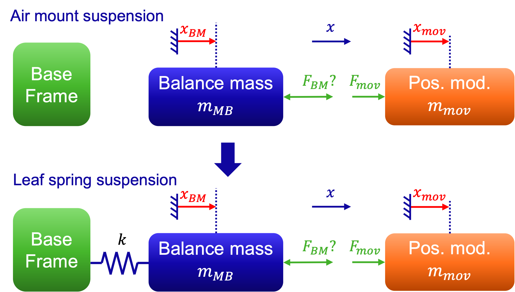
Fig. 5.34 The balance mass in two configurations: top scenario suspended by air mounts isolating it from the base frame, bottom scenario connected via leaf springs with stiffness \(k\), showing how spring stiffness influences vibration transmission to the base frame.#
Derive the equation of motion for the balance mass – leaf spring system as function of \(F_{\rm mov}\). What is the eigen frequency \(\omega_{BM}\) of this system?
Derive a relation for the reaction force onto the base frame as function of \(F_{\rm mov}\)?
Reason how much force is felt by the base frame for the situation \(k \cdot x_{BM} \ll m_{BM} \cdot \ddot{x}*{BM}\) (or equally \(\ddot{x}*{BM} \gg \omega_{BM}^{2} \cdot x_{BM}\)) and for \(k \cdot x_{BM} \gg m_{BM} \cdot \ddot{x}*{BM}\) (or equally \(\ddot{x}*{BM} \ll \omega_{BM}^{2} \cdot x_{BM}\)).
Given that the purpose of a balance mass is to isolate as much force from a moving body towards the ground as possible, which of the two situations is preferred? Would this preferred situation correspond to a relatively small or large stiffness? What would consequently be the desired eigen frequency (small or large)?
Given the range constraint and desired isolation properties of the balance mass, what mass and stiffness (and eigen frequency) advise would you give the mechanical designers that need to design this system?
Vibration isolation tables can be considered closely related to balance masses. These tables are commonly used in precision measurements which require near perfect isolation from the fixed world, e.g., atomic microscopes (Thermo Fisher?), optical setups (companies?), but also CERN and other parts of lithography systems.
An important difference with balance masses is that vibration isolation tables try to isolate the system from ground vibrations. After a change in schematics, see Fig. 5.35 and Fig. 5.36, however, the analysis step from the previous slides can still be used to analyze and/or specify the desired behavior of these tables.
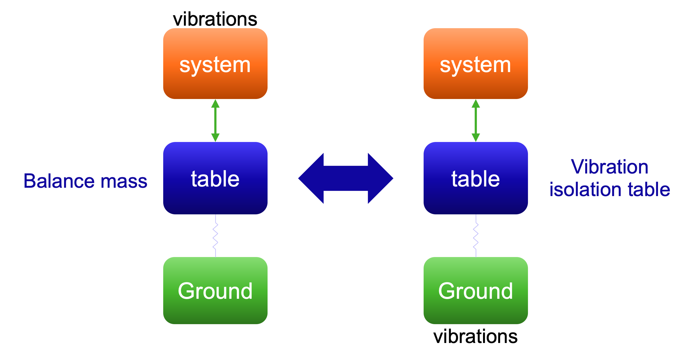
Fig. 5.35 Schematic of balance between mass and vibration isolation tables, showing how both isolate vibrations but with opposite focus—balance masses isolate ground from system vibrations, while isolation tables protect the system from ground vibrations.#
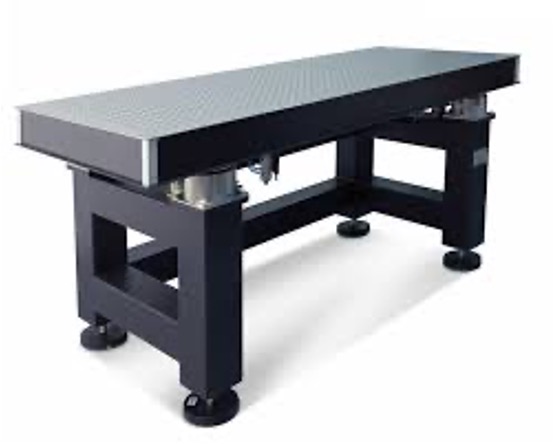
Fig. 5.36 Real vibration isolation table used in precision systems to minimize ground-induced vibrations reaching sensitive instruments.#